So, Which Machine Learning Algorithm Should You Use?

As a data science practitioner, you've probably found yourself scratching your head when trying to choose the best machine learning algorithm for a project. With so many options available, the process can feel overwhelming. Let's simplify it.

Start with a fundamental question: what is a machine learning algorithm actually trying to do? At its core, any algorithm takes a set of features and translates them into a useful prediction, using a mathematical system unique to that algorithm. The translation process varies widely from one algorithm to another.

So what's the keyword that plays the major role in selecting an algorithm? It's simple: the features themselves. You're just trying to choose the best translator for your specific set of features.

In this post, we'll break down the most widely known algorithms based on their general behavior, then walk through how exploratory data analysis and feature engineering point you to the right family — and finally, the non-data considerations that make the final call.

The decision boundary concept

It's crucial to have a clear understanding of the decision boundary concept. The decision boundary defines how an algorithm behaves — how it interprets and processes data. It essentially highlights the strengths of each algorithm, giving you valuable insight into where it will perform well and where it will fail.

The figure below, adapted from a classic sklearn example, shows how different algorithms perform on different toy datasets. Each column is the same data; each row is a different algorithm's attempt to separate the two classes:

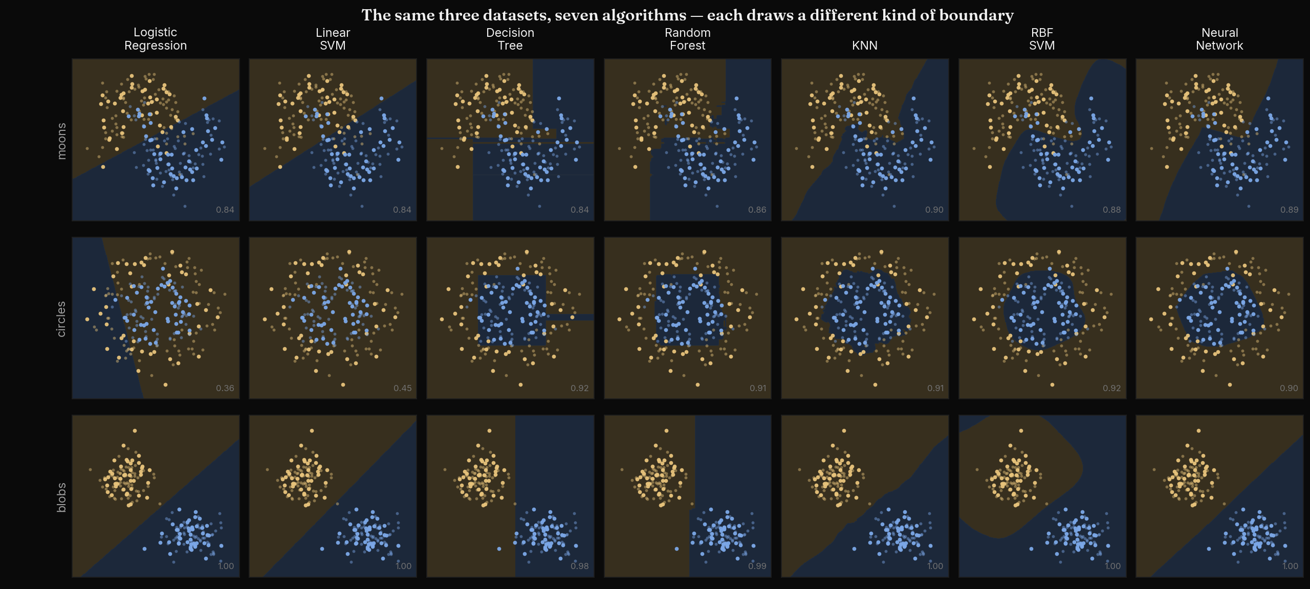Same data, seven algorithms — logistic regression and linear SVM draw straight lines, trees draw boxes, KNN follows neighborhoods, RBF SVM and neural networks draw curves.

This graph is a powerful tool. By examining it row by row, we can see how each algorithm interprets and processes data in a unique way:

• Logistic regression and Linear SVM try to slice the data with a straight line to determine the class of each point. On the moons and circles datasets, they fail no matter how you tune them — the boundary they need doesn't exist in their vocabulary.
• Decision trees and random forests use a strategy of splitting the data with if-then rules to separate classes, with random forest taking this approach further by combining many trees. The result is an axis-aligned staircase of splits — crude for one tree, smoother for a forest.
• Nearest neighbors (KNN) relies heavily on the proximity of data points — it traces the local neighborhood structure, which makes it flexible but jagged and easily distracted by noise.
• RBF SVM and neural networks both aim to find linear combinations that separate the data, but in a transformed feature space rather than the original one — which is why they can draw smooth curves and handle every dataset here well.

Understanding the decision boundary concept is essential for selecting the best algorithm for a particular dataset. Once you know how an algorithm behaves, you can make an informed decision instead of guessing.

The model families

By categorizing algorithms based on how they draw their boundaries, the zoo becomes manageable. There are four families worth knowing:

Four families, four ways to draw a boundary — with probabilistic models like Naive Bayes sitting outside the map.

Linear models

A linear model is one specified as a linear combination of the features. During learning, the algorithm computes a weight for each feature based on the training data, forming a linear equation that maps inputs to the target. Adjusting the weights is the entire learning process. This family includes linear regression, logistic regression, and linear SVM.

One precision worth stating, because it's widely muddled: "linear model" means linear in your input features — a weighted sum of the columns you feed in, full stop. A neural network is not a linear model; it's a composition of linear maps and non-linear activations, which is exactly why it can draw curves. Likewise, an RBF SVM is linear only in an implicit, transformed feature space — in the space where your features actually live, its boundary is curved. That's why those two belong to their own family: learned feature space models. A neural network learns its internal features end-to-end; a kernel SVM's feature space is fixed by the kernel, with only the weights learned — but either way, the model is linear there, not in your columns.

Tree-based models

Tree-based models use a series of if-then rules to generate predictions from one or more decision trees — that's the splitting effect you saw in the figure. The tree starts with a single node representing the entire dataset, then splits into branches based on a particular feature, repeating until each subset is (mostly) one class.

This family includes the decision tree itself plus the ensemble methods built on it: random forest, gradient boosting, XGBoost, LightGBM, AdaBoost, and CatBoost. Single decision trees are simple and highly interpretable; random forests combine many trees to improve accuracy and reduce overfitting; gradient boosting iteratively builds trees that correct the previous ones' errors.

Distance-based models

Distance-based models determine the decision boundary based on the closeness of points to each other. The most popular example is KNN: find the k closest training points to the input and predict the majority class among them. Because everything rests on a distance metric, these models are heavily influenced by the scale of each feature — normalization or standardization is usually required, or your largest-magnitude feature silently dominates every distance.

Where does Naive Bayes live?

You'll often see Naive Bayes filed under distance-based models — I did this myself once, and it's wrong. Naive Bayes is a probabilistic model: it scores each class with Bayes' theorem under a conditional-independence assumption between features. No distances involved. (A nice detail for interviews: with Gaussian, equal-variance features, Naive Bayes is actually linear in the log-odds — mathematically closer to logistic regression than to KNN.)

The key question: splits or surfaces?

With the families in mind, a simple question emerges: are the features in our data more useful for creating linear trends with the target, or for creating splits between classes?

If the features show a clear relationship with the target that can be expressed linearly, a linear model may be appropriate. If the data requires splits to separate classes, a tree-based model is likely more suitable. To answer this question, we turn to exploratory data analysis.

Exploratory data analysis: the cornerstone

EDA is the cornerstone of data science. The ultimate goal is to know, explore, and visualize your data to make informed decisions — and one of the most important decisions it informs is model selection. While there's no rigid process, two steps reveal most of what you need:

Step 1: Summary statistics. Percentiles, ranges, variance, and standard deviation identify where most of the data lives. Averages and medians describe the central tendency. Correlations indicate strong relationships between features and the target.

Step 2: Visualize the data. Box plots identify outliers. Density plots and histograms show the spread of each feature. Scatter plots describe bivariate relationships between features and the target.

Now let's look at how the outcomes of these two steps contribute to model selection.

Outliers

Outliers can significantly impact any linear model — squared loss literally squares their influence, so the model contorts itself to fit points that may not even matter. That raises two questions.

First: is a linear model appropriate given the outliers? Tree-based models are far less affected, because splits will most likely isolate outliers into their own small leaves and move on.

Second: if outliers persist, how do you handle them? You could remove them, but that risks losing valuable information — in some cases outliers are a golden feature with strong predictive power (think fraud). Clipping helps linear models but destroys information by flattening real extremes. Transformations like log or square root add a damping effect to large values without information loss, which is why they're usually the better companion for linear models. The handling method should be chosen based on your specific data and the model family you're leaning toward.

Data distribution and correlation

Two factors matter here: distribution shape and correlation strength.

One correction to a claim you'll see everywhere (including, once, from me): linear regression does not assume your data is normally distributed — it assumes the errors are, and only for valid confidence intervals at that. What actually matters for model choice is the shape of the feature–target relationship. If the data is heavily skewed or the relationship is non-monotone, tree-based models are a natural fit, because splits don't care about the shape of any distribution.

Correlation strength is the second signal. Strong, monotone correlations between features and target favor linear models — they'll capture the signal with a handful of coefficients where a tree needs dozens of splits. Weak or interaction-heavy relationships favor trees, which are far less affected by weak individual correlations.

Missing values

When missing values are present, a few questions determine the best approach.

First: are the missing values related to a specific event? If so — "income missing = applicant declined to disclose" — the missingness itself is signal. Treat it as a separate category, which tree-based models handle beautifully by splitting on it.

If a linear model is still required, the question becomes which imputation technique minimizes damage to the feature–target relationship: mean, median, or something more sophisticated like KNN imputation.

Another option is a model that handles missing values internally. XGBoost routes NaNs down learned default branches at each split. Naive Bayes can simply skip the missing feature's likelihood when scoring — though be careful: sklearn's implementation rejects NaNs outright, so this requires manual implementation.

Feature engineering follows the model family

Once EDA gives you a sense of direction, feature engineering should be done with respect to the model family you'll use. The preprocessing that helps one family is wasted on another.

Missing value handling

• Imputing categorical missing values with an explicit "Unknown" category benefits tree-based models, which can split on it directly.
• Imputing with mean or median benefits linear models, because it preserves the linear relationship between variables instead of injecting an artificial level.
• Models that handle missing values natively are not magic — unhandled missingness still degrades their performance, as with the Naive Bayes caveat above.

Scaling and normalization

• Tree-based models: not affected at all. They work by recursively splitting on feature values, so the relative scale of features is irrelevant.
• Distance-based models: profoundly affected. Scaling ensures every feature is equally important in the distance computation — otherwise one large-scale feature dominates the metric and biases every prediction. (Occasionally you'll even deliberately not scale a feature to make it dominant, but that should be a conscious choice.)
• Linear models: scaling doesn't change what an unregularized fit can express, but it speeds up gradient-based solvers significantly, reduces the impact of outliers, and becomes non-negotiable once regularization enters — the penalty treats large-scale coefficients as more important.

Categorical variables

• For linear models, one-hot encoding transforms each category into its own binary column, letting the model learn a separate weight per category with no fake ordering imposed. Frequency encoding — replacing each category with its frequency in the dataset — compresses high-cardinality features into one informative column that captures the category distribution.
• For tree-based models, label encoding creates an ordinal relationship that boosts the model's ability to split, and some implementations (CatBoost, LightGBM) consume categoricals natively. Target encoding — replacing each category with the mean of the target for that category — captures the category–target relationship directly, but fit it on out-of-fold data or you'll leak and overfit, especially with rare categories.

Get the family right and much of "feature engineering" becomes obvious. Get it wrong and you'll spend a week tuning around a mismatch that a different algorithm would have made disappear.

Deployment considerations

After EDA and feature engineering point you toward a family, it's important to consider factors unrelated to the data itself:

• What is your storage capacity? A random forest with hundreds of deep trees, or a KNN that must carry the entire training set into production, can be a genuine deployment problem on edge devices or small servers. A logistic regression is a handful of coefficients.
• Does the prediction need to be fast? In real-time applications, predictions must be generated as quickly as possible — road signs in autonomous driving must be classified rapidly to prevent accidents; fraud must be scored before the transaction completes. Scoring a linear model is a dot product — microseconds. A large ensemble costs orders of magnitude more.

Explainability vs. predictability

Finally, the trade-off every data scientist should keep in mind. Explainability is the extent to which we can explain the model's prediction: a decision tree is highly explainable because you can follow the exact sequence of if-then rules that produced any output. These are the "white-box" models. Predictability is the model's raw ability to make accurate predictions, regardless of whether we can explain how it arrived at them. Neural networks sit at the far end — very complex, very hard to interpret. These are the "black-box" models:

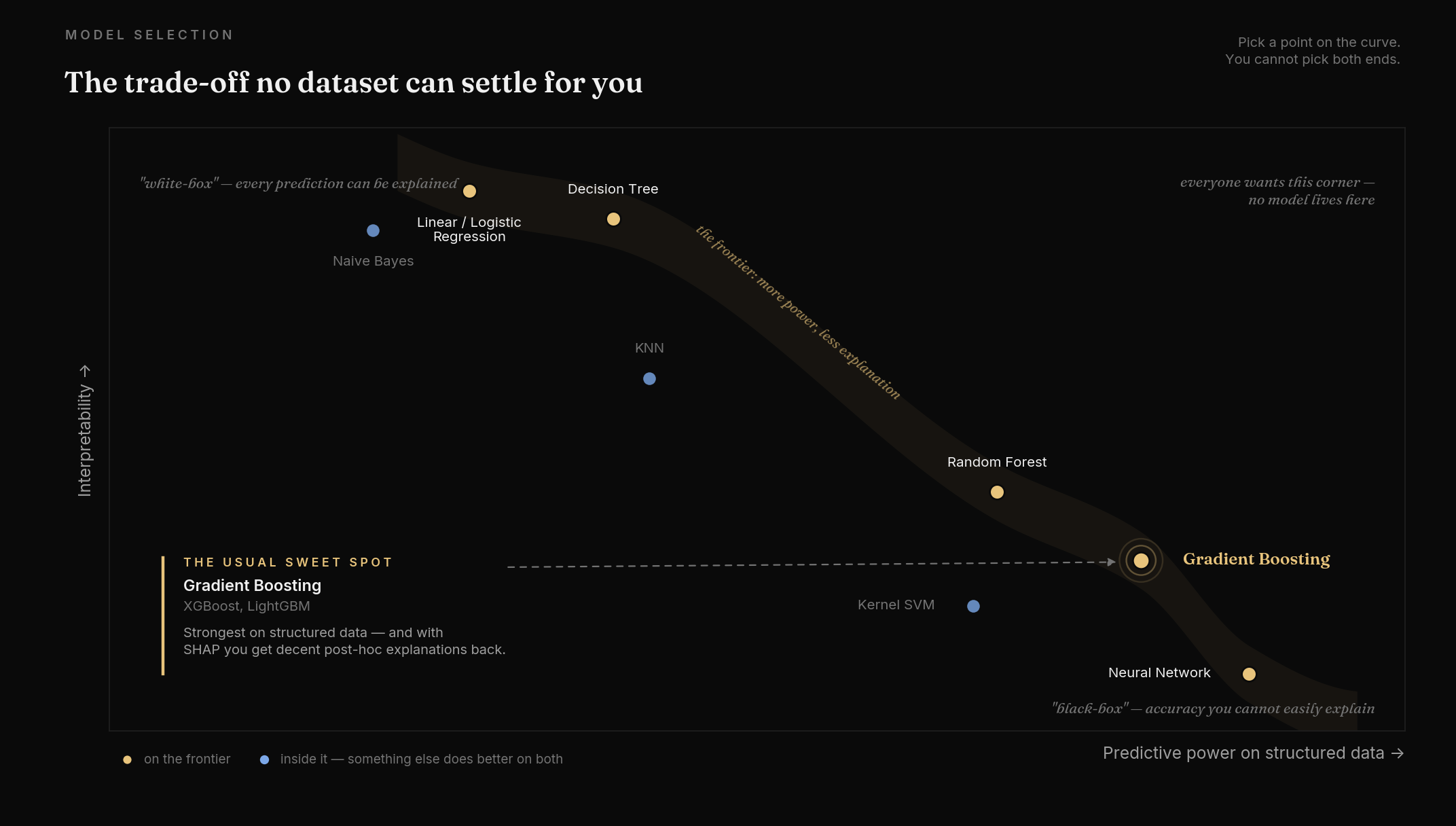White-box models explain every prediction; black-box models buy accuracy with opacity. Gradient boosting is the usual sweet spot on structured data.

Keep this trade-off in mind because some applications require explainability — regulated industries, tools whose users must audit each decision — which means opting for simpler models no matter what the accuracy numbers say. In other situations explainability doesn't matter, and prioritizing raw predictive power is the right call. Notice where gradient boosting sits on the chart: near the top on predictive power for structured data, with SHAP values offering a decent post-hoc explanation. That balance is exactly why it's the workhorse of applied machine learning.

Putting it together

Choosing an algorithm is not a guess or a default — it's a reading of your data:

1. Understand decision boundaries — each algorithm can only draw certain shapes, and the shape your data needs eliminates half the zoo immediately.
2. Do the EDA — outliers, distributions, correlations, and missing values each vote for a family.
3. Engineer features for that family — scaling, encoding, and imputation only help when matched to how the model actually works.
4. Respect reality — storage, latency, and explainability requirements can overrule whatever the data suggested.

The best algorithm is rarely the most sophisticated one. It's the one whose assumptions your data actually satisfies — and that your system can actually run.